Distance on the label is a link budget, not a promise
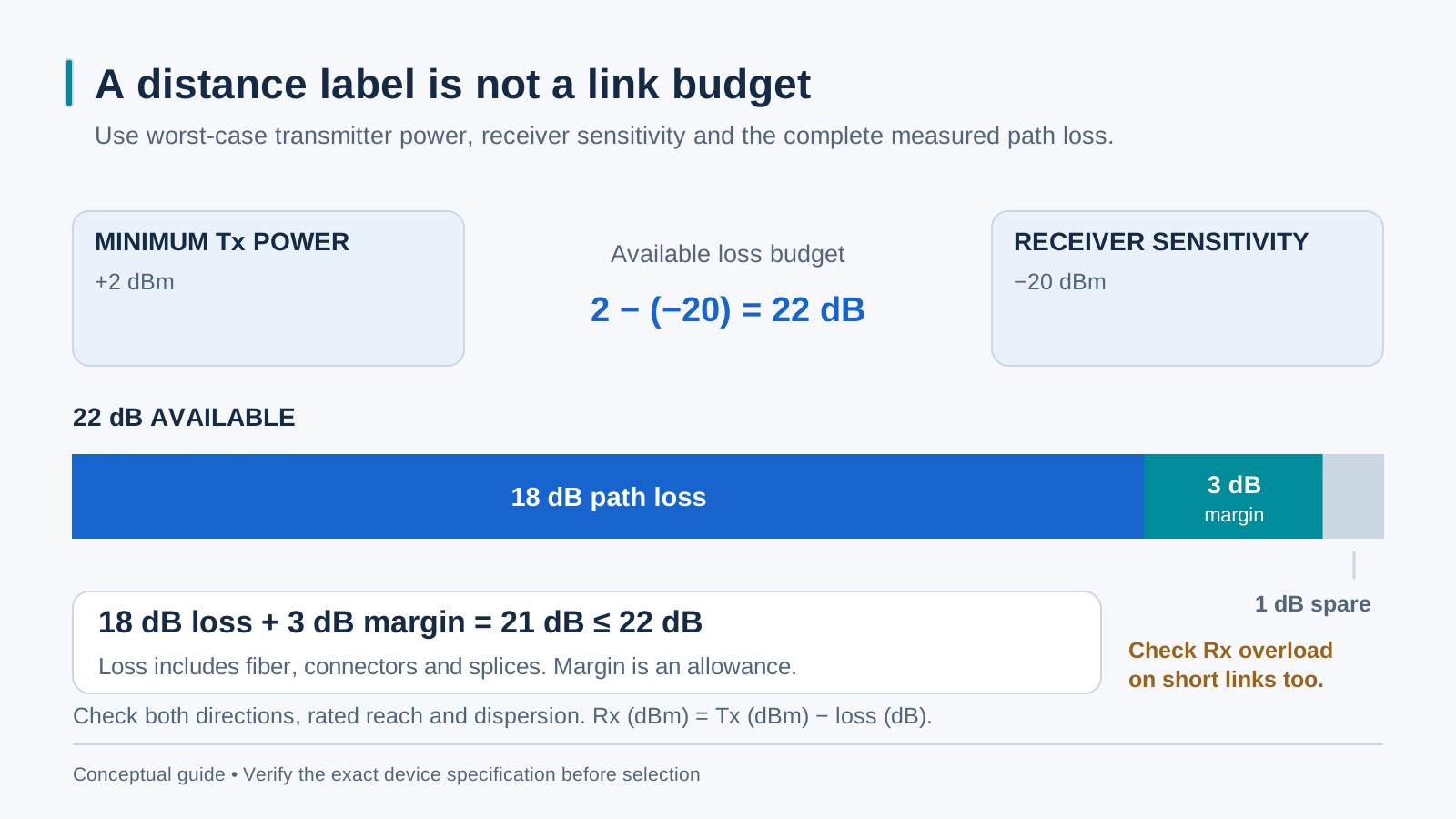
A module’s rated distance applies under its specified fiber and optical conditions; it is not a universal reach guarantee. Calculate the worst-case power budget from minimum transmitter output minus receiver sensitivity, in dB. Account for fiber, connector and splice loss plus a documented design reserve. Also check maximum receiver input, minimum path loss and the optic’s rated reach and dispersion limits in both directions.
1310 nm vs 1550 nm — and the A/B pair
Many single-mode optics use 1310 nm or 1550 nm, with different attenuation and dispersion characteristics. BiDi optics use complementary transmit and receive wavelength bands on one strand. For example, one product pair may use TX1310/RX1550 and TX1550/RX1310, while other families use different bands. Read the actual module specifications rather than assuming that A/B letters define universal wavelengths.
The standard distance classes
Optical interface standards and vendor reach options are different labels. Commonly sold single-mode reach options include 10, 20, 40 and 80 km, but these are not four universal IEEE Gigabit classes. Multimode reach also depends on the optic and fiber grade. Select an interface supported by the host and rated for the intended fiber, distance and optical conditions.
Worked example: budgeting a 42 km link
Illustrative assumptions for a 42 km route at 1550 nm: 42 × 0.22 dB/km = 9.24 dB of fiber loss; two connector pairs at 0.5 dB add 1.0 dB; four splices at 0.1 dB add 0.4 dB; a 2 dB repair reserve gives 12.64 dB in total. These are example allowances, not measured site values. Select an optic rated for the route and verify both directional power windows and dispersion. Do not approve a 42 km route from loss arithmetic alone, or assume that a higher-power optic is always safer.
Multimode vs single-mode
Multimode and single-mode fiber require compatible optics and launch conditions. Jacket color can be a clue, but confirm the cable marking, fiber grade and test records. Connector type alone does not prove compatibility: an LC connector can be used on different fiber types. Some LX/LH optics support specified multimode links with mode-conditioning guidance; follow the selected optic’s documentation.
Five mistakes that kill long links
Common planning mistakes include using map distance instead of the cable route, omitting connector or splice loss, choosing incompatible BiDi wavelengths, ignoring receiver overload, and skipping link testing. Use surveyed route length or certified test results rather than a fixed multiplier of road distance. Verify the optical specifications at both ends and measure the installed link.
Pre-deployment checklist
Before ordering, record fiber type and grade, actual route length, connectors and splices, the optical standard and wavelength pair, and the required design margin. Verify both sensitivity and overload limits and any dispersion or minimum-distance restrictions. After installation, record received power in dBm at both ends and path loss or margin in dB, and label the endpoints consistently.